Buddhabrot, domain coloring, fractal flames and nevroses
For the past year or so, I have been working on a buddhabrot using the lambda function, defined by
$$ f_r(z) = r * z * (1 - z) $$
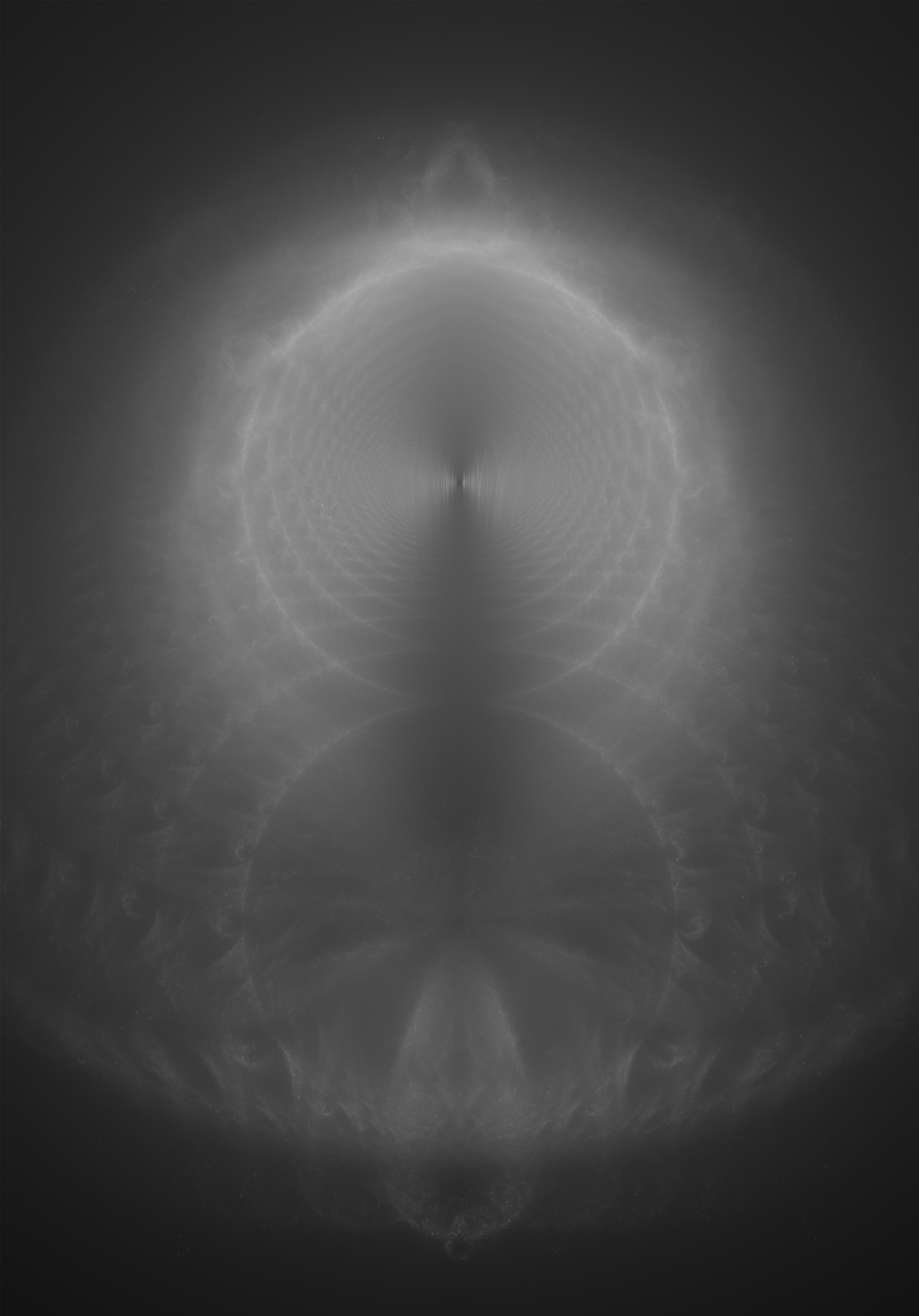
With \(r, z \in \mathbb C\). The goal initially was to simply compute an image (which I will refer to by the Buddhalog from now on) using the Buddhabrot technique, created by Melinda Green. A buddhabrot is a way to show the trajectories of points under iteration of a map: it’s an histogram of trajectories. The “classic” buddhabrot uses the world-class mandelbrot function: \(f(z) = z^2 + c\) with \(z, c \in \mathbb C\). The algorithm is roughly as follows:
Create a 2D int array of size NxM
for n = 0; n < num_pts; n++
	c = random complex
	for i = 0; i < maxiter; i++
		trajectory[i] = trajectory[-1]**2 + c
		if |trajectory[i]| > 2:
			for p in trajectory
				px = map \\(\Re(p)\\) from [-2; 2] to [0; N]
				py = map \\(\Re(p)\\) from [-2; 2] to [0; N]
				histo[px][py]++
			break

for x, y in N,M
	color_image[x][y] = log(histo[x][y] + 1)/log(max(histo) + 1)
You then have a 2D array filled with values between 0 and 1, which you can then map to intensities. The Buddhabrot creates a very nice and fine image, with a bunch of details and smooth gradients. However, it is very expensive to compute. In essence, we are trying to approximate the probability distribution of points that escape under iteration of the mandelbrot function. The more iterations we do, the better the details, but we then need much more points to sample, as the regions where points attains those high iterations counts becomes much smaller (and approximate the Mandelbrot set). Almost all points will either diverge very rapidly, or get sucked in a cycle.
Another aspect to consider is that a computing Mandelbrot set is very easy to parallelize. Each pixel can work idependentely of each other, and the result of the function on each pixel is the final color. The color of a pixel on a Buddhabrot is the results of hundreds of thousands of iterations, and different points. It’s very slow. An image might take a few hours (or days !) to just begin to show if you have made a mistake, whereas with other processes (like a complex bifurcation diagram, the build iterations are much faster. This is even worse in our case, where we need to sample 2 complex points: \(r\) and \(z_0\), or 4 reels. The sampling region is also fairly important, and the larger the better (but this has diminishing returns). I sampled \(r\) and \(z_0\) with real and complex part in [-5; 5].
Disgression into Client-Server and histogram normalization.
I created a simple screensaver (that might or not work for you), that I would install on my machines, and they would compute a bunch of trajectories, combine them into an histogram and send them to a server. The server would add all the histograms together, and create the final image.
I threw some code together and with the help of a good friend, we managed to set up everything needed. My computers chugged along, and over the course of a few months and messed up runs, I had an image.

This is about a 100 billion sample, done over the course of 2-3 months. The fractal is log-scaled, as a linear scale was destroying details. The distribution of values in the histogram (the histogram of the histogram if you will) is actually very heavily long tailed, with about 99% of values being under 2000, but a single point having a value of more than 40k. This means that normalizing the histogram by dividing all values in the histogram by the maximum would set as 0 or very close to 0 almost all values. A log transform is actually not quite the best, and tends to create images that are a bit too “smoky”, with low values being overrepresented. I don’t like to use alpha correction as it tends to clip heavily on this image and create big blobs of all white values which does not look too good. However, it is possible to make the image “pop” a bit more, by clipping values over and under a threshold and then remapping to 0-255; or just playing around with the “curves” tool in Gimp.
Colors: Fractal flames and domain coloring
So there I was. After pretty much half a year, I had my image, with the correct function, and in the correct format. All done. I just wanted to see if I could color it nicely, and 6 months later I’m still computing this image.
The classic way to color a Buddhabrot is to use different maximum iteration counts for each channel. An RGB image is just an array of NxMx3 integer values between 0 and 255. For example the R channel is would be Buddhabrot computed with 100K samples and 100 iterations, the G channel 100K samples and 1000 iterations and the Blue channel would be 100K samples and 10K iterations. This create false colors which do look great, but I always felt that this was a bit too artificial. The final color will be an obvious choice by the programmer, with channels with a higher iterations counts dominating the others. I wanted the color to show something meaningful.
The fractal flames algorithm gave me the idea: on top of having a 2D histogram, you also compute a RGB array. Each time you iterate using a function, you update the value in the histogram in the corresponding cell, but also update the color by setting it as the mean between the current value and the color of the function. Once all the points have been sampled, you log normalize the histogram, and the RGB value of each pixel is multiplied by the value of the histogram. Cells where a lot of points passed by will have brighter colors than others.
With fractal flames, the color of the function (or variation) is set randomly. There is however another: domain coloring. Domain coloring allows visualisation of complex functions, by assigning each complex value a color. We use the HSV model, instead of RGB, as it is more natural. The Hue is derived using the argument, and the Value is computed using some function \(f\) of it’s modulus \(r = |z|\). I used \(f(r) = r^4/(1 + r^4)\).
I decided to only use the \(r\) parameter for the coloring, and not the initial starting value \(z_0\), altough it would be understandable to use both (maybe by getting the color of \((z_0 - r) * 1/2\) ?). Here is a rough overview of the algorithm, with period checking:
histo = 2D int array of size NxM
histo_color = 3D int array of size NxMx3

for n = 0; n < num_pts; n++
	r = random complex
	z0 = random complex
	color = domain_coloring(r)
	period = 0
	oldPoint = -10 - 10i
	for i = 0; i < maxiter; i++
		trajectory[i] = r * trajectory[-1] * (1 - trajectory[i - 1])
		if |trajectory[i]| > 2:
			for p in trajectory
				px = map \\(\Re(p)\\) from [-2; 2] to [0; N]
				py = map \\(\Re(p)\\) from [-2; 2] to [0; N]
				histo[px][py]++
				histo_color[px][py] = (color + histo_color[px][py])/2.0
			break

		if |trajectory[i] - oldPoint| < EPSILON
			break

		if period = 16
			period = 0
			old_point = trajectory[i]
		period++

for x, y in N,M
	color_image[x][y] = histo_color[x][y] * log(histo[x][y] + 1)/log(max(histo) + 1)
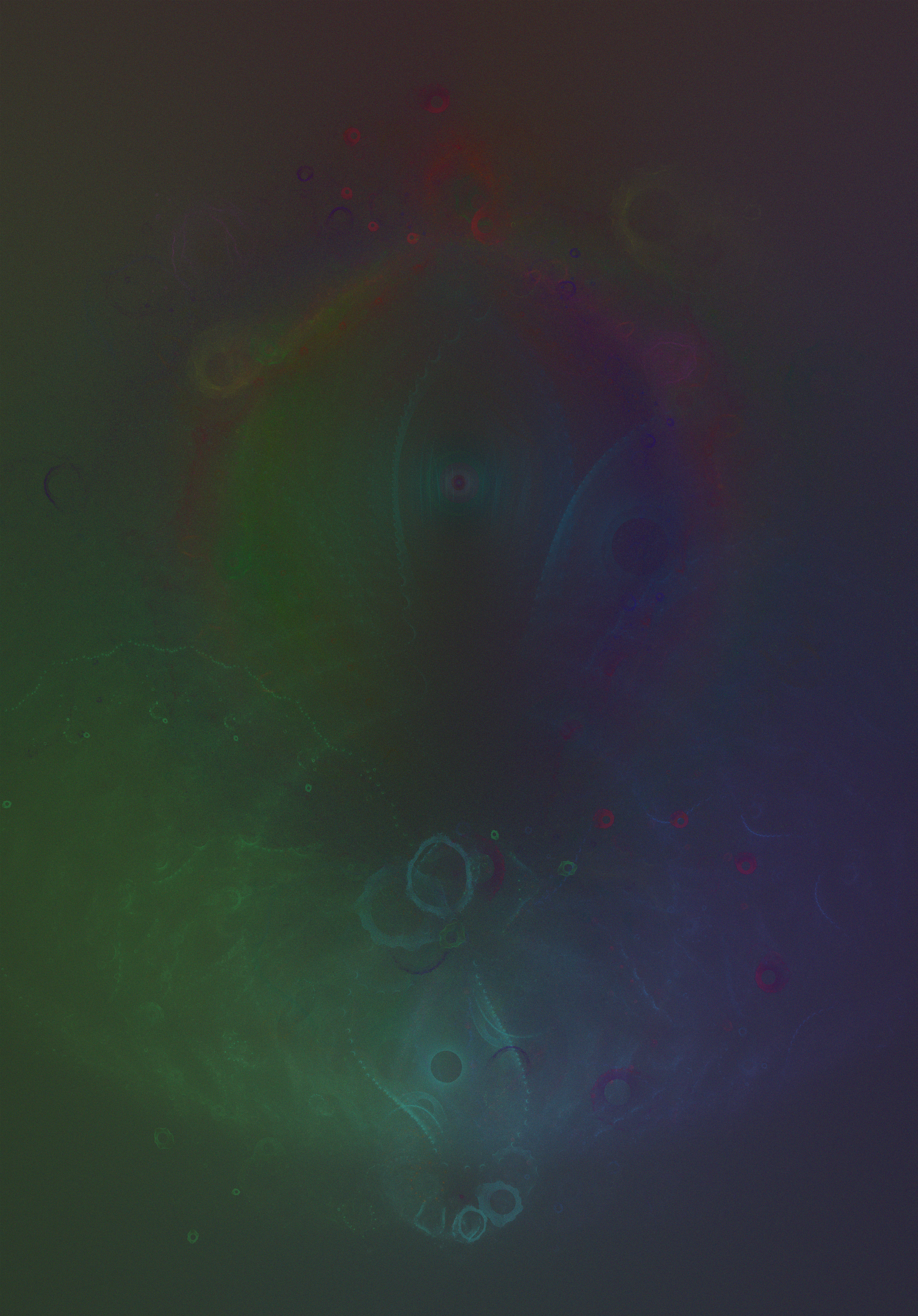
Here’s the final result.

Computing this required some tricks, as it is not a simple elementwise addition of arrays. I re-used my client-server computing platform, and made some slight modifications. The client compute about 100K “good” samples (i.e. trajectories that have more than 16 points), so that we don’t spend our entire time recuperating and sending our work. The histogram is computed naturally, by addition of the received histogram and the current one. However, the client also sends the RGB values of the image. Here, we can’t just find the mean between the received RGB array and the current one, as there is a bunch of black pixels in the received arrays. We would simply end up dragging down the value of every pixel in the current array simply because the received array is mostly empty. On the opposite side, we can’t just find the mean between all the non zeros element of the received array, because a bunch of element in the current array are 0 (especially at the start). This would basically divide by 2 all “new” elements (i.e. those that replace a 0 element in the current array). This division has already been done when computing the trajectories, so this is just redundant. In case of 0 element in the current array, we simply replace by the received element. If both element are non zero, we replace by the mean of those two elements.
This method obviously needs even more samples than the regular one, so some “blemishes” or very high iteration count trajectories are visible. It would seem kinda obvious that the traditional method of random sampling is not quite enough to efficiently approximate this probability distribution.
As a parting gift, here is Buddhabrot colored using this technique. It used 100k maximum iterations, and a few millions points. The coloring is based on the domain coloring of the \(c\) parameter. It obviously needs more baking time, which I might do sometime.
