Complex Plots of Fixed Points of Iterated Polynomials

A fairly long title for this one, but I can’t always be Victor Hugo when it comes to posts titles. We’re gonna talk about complex dynamics in this one, so stay strapped.

When I first started learning about Discrete Dynamics, an exercise that would often come up would be to find the fixed point of the nth iteration of the logistic map, or put it simply solving the following equation:

$$ f^n(x) = x,\\ f^n(x) = \underbrace{f \circ f \circ … f(x)}_n$$

With \(f(x) = rx(1-x), \; 2 > r > 4\). Yes I learned how to use \underbrace just to get this nice formating. Another way to put the first equation is as follows:

$$ f^n(x) = x \Leftrightarrow f^n(x) - x = 0 $$

Anyway, this is our day of luck, since if you look a bit carefully, you notice that \(f\) is a polynomial. This means that the right part of the equivalence above is also a polynomial, and we will have \(deg(f)^n\) solutions. This means that we are guaranteed to find a n-cycle for each iteration number. They might not be unique, but they will be there.

However ! Anyone who looked at a bifurcation diagram will immediatly jump on their chair and say that, for low values of \(r\), the logistic function converge toward a fixed point under iteration and kinda stays there. Does it means that every solution is the same ? If not, where are they, what are their name, what is the profession of their parents ?

Turns out we’re only seeing a small sliver of the logistic function. Since it’s a polynomial, it is essentially a complex function, but we’re constraining it to the real numbers. The other solutions are hiding in the complex plane !

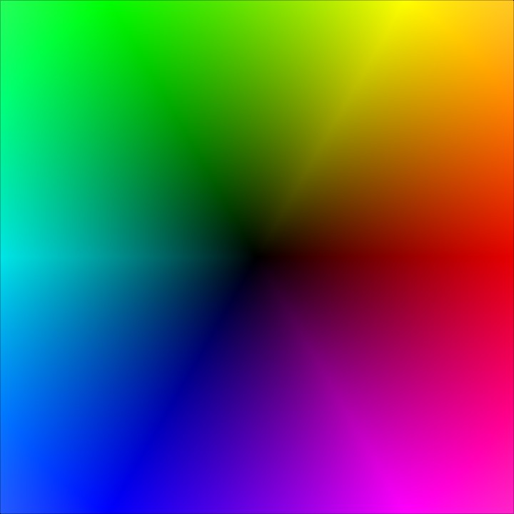
We can visualize actions on the complex plane using a really neat trick called domain coloring. We assign a color to each point on the complex point using a color function. Using the HSL color space, we assign the hue based on the argument of the point, and the brightness using a color function, like \(\frac{2}{\pi} arctan(r)\). The Image below shows the identity function plotted using this type of visualization. It looks pretty.

Enough talk. The video below shows the position of the fixed points of the second iterate of the logistic map, with the \(r\) parameter moving from 2 to 4. The fixed point are represented as black values. You can see the fixed points moving toward the real line. At a certain value of \(r\), all fixed points are on the real line, and this is where the bifurcation happens.

On higher iterations count you can see that the number of fixed point (well, cycles here) grows quite dramitically, and forms some kind of hull. As the \(r\) parameter increases towards 4, this hull squishes towards the real axis.

They do look a bit like julia maps, don’t they ?

I’d be interested to see what actually happens during the stable regions of the logistic map, and what does it mean for the zeros.

Also, you can do this with any kind of complex iterated function. The logistic function is a nice one since it’s a polynomial so you’re kinda guaranteed to find stuff and also because I don’t really recall ever seeing a generalized complex log map. This is a hint toward a future post.