Indra's Pearl, or Quasifuschian Two Generator Groups explained by someone completely out of his depths

A few months back I started reading Indra’s Pearl by Mumford, Series and Wright. The book is amazing, and I’m not scared to say it’s one of my favorite books about Maths that I’ve ever read. I wanted to get my hands dirty and implement some of the fractals in the book, since they were very different from the usual “Mandelbrot and cousins” fractals: they were truly out of this world. So I did ! But turns out I couldn’t just do a few techniques, I had to do them all.

In this series, I’ll try to explain succinctly what exactly are Indra’s Pearl, why my program is named “ceendras pearl” (it’s because it’s in C, there isn’t much to it actually) and what kind of great stuff you can do with it. A note: all figures are reproduced from the book, but I’ve drawn them myself to not attract the wrath of the copyright holder. The fractals are made using my program, so I should be safe(r).

You can do this !

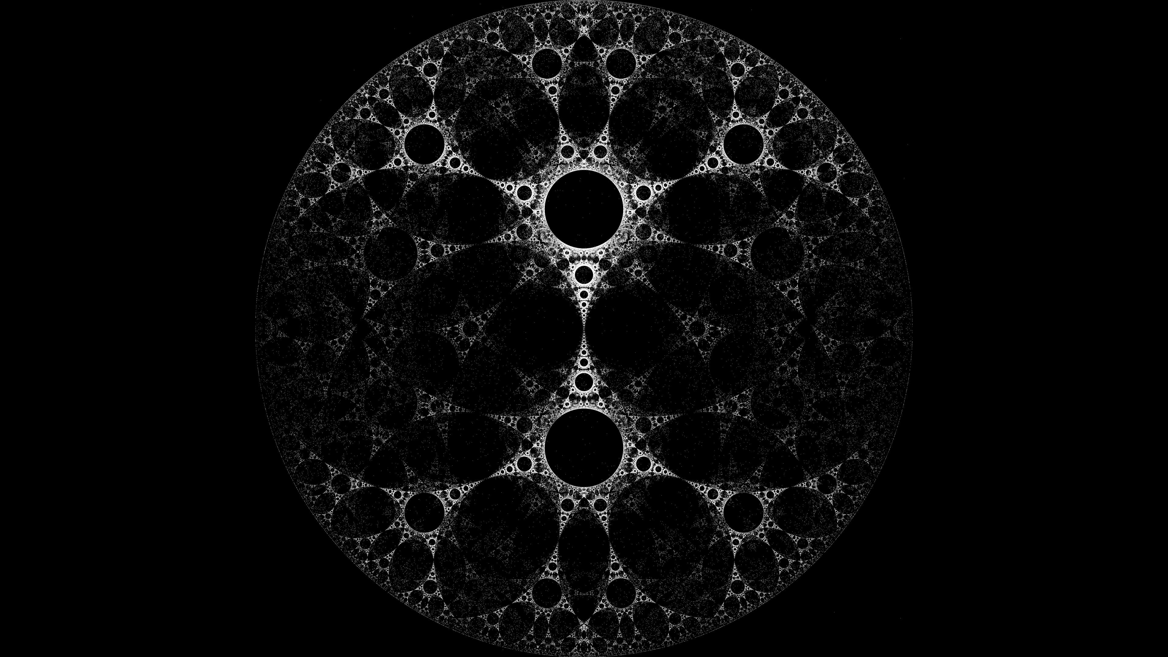
Cool heh ? Well you too will be able to do this crazy stuff using Ceendras Pearl, the leader in Klein Fractal Computator ! Just 300 low low payment of 0.0$ will net you those crazy fractals ! It’s an Epsilon GUARANTEE !

What exactly are we doing ?

At it’s heart, Indra’s Pearl is about exploring the words of a group of 2 (or more) generators, which are Mobius Transform. We do this using a Depth First Search on the tree of words, and after bailing out we are plotting the limit set of those groups.

There is a lot of stuff we can do with them. Even choosing some random parameters and plugging them into the program gives out some great results. There is also some very deep relations to a wide variety of mathematics topics, along with some from computer science. Essentially we are doing iterations with multiple functions, which are very special and with a ton of useful properties tacked on to them.

We can create a more generalized version of Appolonius Packing, we can use newton method to find a special root of a characteristic polynomial associated to a fraction, which gives us a parameter to create our fractal with, we can approximate irrational groups, with cusps and degenerate space filling weirdness. There’s something for everyone, even just the dude who just wants to look at pretty images, and doesn’t want to think about Four times punctured sphere, or Teichmüller Theory.

There might even be a way to define this sort of plots for quaternions, and create a 3D version of the object we will see here, but I haven’t given that much thought.

That’s a lot of stuff to define, so let’s get to it right away !

Groups

A group is defined as a set, equipped with a binary operation ($*$) that combines two element of the group to form another element of the group. It must also satisfies the following conditions: - Associativity: $(a * b) * c = a * (b * c) $ - Identity: There must be an element $e$, such that $e * a = a$ and $a * e = a$. $e$ must also be unique - Inverse: For all element $a$ in the group, there must be an element $b$, such that $a * b = e$ and $b * a = e$, with $e$ being the identity.

In our group, our elements will be Mobius Transform and we’ll define the binary operation as the traditional matrix multiplication. So, every time you see $*$, think “matmul” or “@”. A word is defined as the product of the elements of the group and their inverse. For example, $abAB$ is a valid word. We basically want to explore all the words that can exist.

Something that will interest us greatly are the limit sets. Those sets are the “end products” of infinite words.

Möbius Transforms

Möbius transforms are a very important part of complex analysis. They look like this:

$$ f(z) = \frac{a z + b}{c z + d} $$

With $a, b, c, d \in \mathbb{C}$. Möbius transforms are nice because they map circles to circles, and lines to lines. They themselves form a group. Möbius transforms multiplied by another Möbius Transform gives another Möbius Transform. And of course each of them have their own inverse. You can see them as a $2 \times 2$ matrix with complex coefficients.

$$ \frac{a z + b}{c z + d} \leftrightarrow \begin{bmatrix} a & b \\
c & d \end{bmatrix} $$ Applying a Möbius Transform to a point is now considered as a simple matrix multiplying a vector. We can categorize Möbius Transforms by the trace of their respective matrix. The trace $tr$ is the sum of each element in the diagonal of a matrix T, so here $tr(T) = a + c$. There are four kinds of Möbius Transform in this categorisation, each with funky names:

Loxodromic ($tr(T) \notin [-2;2]$) : Those Transforms have two fixed points: one source and one sink. Points move in spirals around those points.
Hyperbolic ($tr(T) \in \mathbb{R},Tr(T) \notin [-2;2]$) : Special case of Loxodromic transforms, where points move in circles through the two fixed points.
Elliptic ($tr(T) \in \mathbb{R}, Tr(T) \in [-2;2]$) : Two neutral fixed points, and points move around in circles around those fixed points.
Parabolic ($tr(T) = \pm 2$) : One fixed point which is both a source and a sink. The most interesting of them all !

Here, fixed points, sinks and sources have the usual definition, which I’ll recall rapidly. A fixed point is a point that stays the same after application of a transform. A source “repels” points close to it under repeated application of the transform, while a sink “attracts” points near to it. Of course, a transform who operates on a dimension higher than 1 can be both, attracting and repealing points on different axes.

Schottky Arrays: Getting into the meat of it

The first funky thing we can do is create a Shottky Array. We craft two Möbius Transforms which pairs circles together and apply those transforms repeatedly.

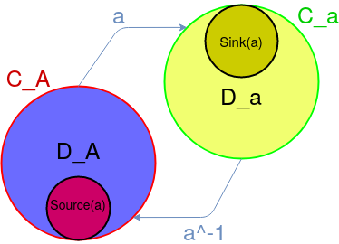
A loxodromic transform pairs the circles $D_A$ and $D_a$ if it respects the following conditions:

The disks $D_a, D_A$ do not overlap
The outside of $D_A$ is mapped to the inside of $D_a$, and the inside of $D_a$ is mapped to the inside of $D_A$
The circle bounding $D_A$ is mapped to the circle bounding $D_a$
The sink of $a$ is inside of $D_a$ and the source of $a$ is inside of $D_A$
Successive applications of $a$ shrinks $D_a$ to smaller and smaller disks all containing the sink of $a$ while successive application of the inverse of $a$ shrinks $D_A$ to smaller and smaller disks containing the source of $a$

A nice illustration of the above principle

It’s quite funny to see the usual definitions of non linear dynamics used in this sense. What we basically do here is create a particular map, with two fixed point, a source and a sink, which are placed in two separate circles. Upon application of this map, the circles converges towards the fixed point of the transformation.

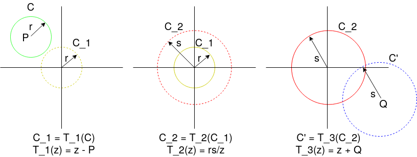
The position of the initial circles will directly impact how the circles will look after iteration. What we do is apply the circle pairing Möbius Transform to a circle $C$, which will pair it to a circle $C'$. This transform maps the inside of a circle to the outi, which can be broken down in three simple steps. T:

First translate the circle $C$ center $r$ to the origin, call this translated circle $C_1$
Then invert the inside of $C_1$ to the outside of another circle $C_2$ also centered at the origin
Finally translate the outside of $C_2$ to the outside of the final circle $C'$

Mobius Pairing

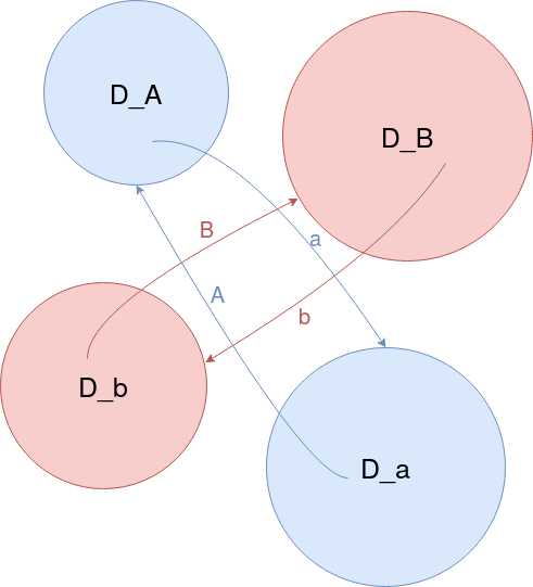
Now for the trick: we use not only one, but two transforms. We now have not 2 but 4 circles. $2 + 2 = 4 $ everything is still alright. Instead of applying the same mapping $a$ over and over, we will apply $a$ and $b$, another transform that also pairs circles to circles.

Dance !

Exploring Words

In essence, we chose (very carefully) two Möbius Transforms, each with very specials symmetry and traces that pairs circles together, compute their inverse, and then compose words with them. Our group is the set ${a, b, A, B}$ with $a * A = Id$, and our operation is the matrix multiplication, since it’s equivalent to multiplying two Möbius Transforms. Creating a word is simply multiplying two elements together. For example, we can create the word $ab$ by multiplying a and b. Quite simple.

Our rule is that we won’t apply the inverse of an element just after applying the element itself. This means that words like $aA$ or $abaaaBBBAAbAAbbAABBb$ are not valid, since we have multiplied together an element and it’s inverse, which means that the word is simply the identity.

We now want explore all words that can be made in this manner. This can be seen as exploring a tree.

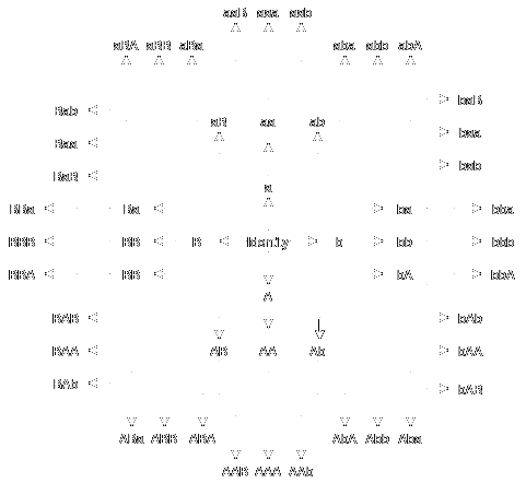
I spent a lot of time trying to make this look fairly good. If you can read this, apocalypse has happened and you can’t see it. I’m very sad. However, if you can’t read this, it means that the image is parsing okay, and you can’t see the effort I’ve made writing this text. Can’t have everything I guess.

We can then (finally !) start plotting some stuff. The easiest way to do that is to do a simple breadth first search on the word tree, and plot the circle associated to each word. We can stop the BFS once we have reached a maximum level in the tree, or when the circle radius is less than an $\varepsilon$. This type of plot is called a tiling plot, and is pretty great, but can get quite messy.

The algorithm for BFS is fairly simple:

For each generator, compute the result of the matrix multiplication with every other generator, except its inverse. Place the result of those matmuls into a word array.
For every element in the array, compute the result of the matrix with every generator, except the inverse of the last generator used. Place the result of those matmuls at the end of the word array. Draw the associated circle using the procedure described above.
Repeat ad nauseam

Of course I’m jumping over some subtleties over how we know which generators we have used last, and how to prevent cancellation.

Above, I am using a parametrised group to produce my generators, which I’m then iterating. For each frame, I am computing a new group, and exploring all words up a certain level. This one is quite messy so I’m not going too far in the exploration, up until the level 9, which is still $4 + 3^9 = 19687$ different words, each with their specific circle.

The BFS algorithm is quite slow, and also is not able to plot the limit sets. As you can see, using a particular set of generators, the circles shrink toward some kind of line. We’d like to just see this line, instead of the huge mess of circles going all around. Also, this line is sometime continuous, and sometimes broken into multiple part. Limit sets who form a circle are called Fuschian, but they sometimes form a quasicircle, which is a circle who has a fractal dimension, and are then called Quasifuschian, which is a really cool name.

Circle, Quasicircle, Fuschian, Quasifuschian and other nice words to win at Scrabble with

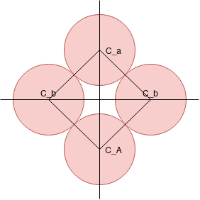
We can create quasifuschian limit sets by pairing Schottky Circles and making them touch at one point. They are then called kissing Shottky groups (cute!).

The above figure shows a simple kissing Schottky group. The original Schottky circle $C_a, C_b, C_A, C_B$ are nicely placed so they just barely touch (or give themselves a light peck I guess). Then, we start iterating. Each original circle got then 3 sub circle, corresponding to a word of length two. Doing this process again will create 3 sub sub circle in each sub circle, each corresponding to a word of length 3. Doing this again… You get the picture. You should also notice that how the sub circle are placed matter. Circles corresponding to words where just one generator is repeated, like $bbbbbbb… = \bar{b}$ kinda stays in the middle, while circles corresponding to words where a different generator from the first is repeated comes closer to its corresponding circle, like $b\bar{a}$. This is reminiscent of symbolic dynamics ! Words which share a long “stem”, the first part of the word will have their circles close together. This also means that $a\bar{b} = b\bar{a}$. This is where the (quasi)circle segments join.

You can create perfect circles by simply choosing kissing Schottky circles sharing the same radius, and placed on a square, like so:

just a square a some circle

The below animation shows a width first exploration of a kissing Schottky array, with the initial Schottky circles placed to create a Fuschian group. Each frame increases the maximum depth of exploration, from 1 to 10. We can start to see a perfect circle forming following the ever shrinking circles.

kiss v2

But I haven’t given a very useful piece of information here : how can we chose the correct Möbius Transforms ? If we just get random matrices, we just get a big mess. Is there a machine capable of blasting us with good Möbius Transforms on demand ? Or maybe, some kind of… recipe ? Yes there is, but this is getting out of hand ! I’ll talk about it in another post.

top