Indras Pearl III : Searching for a place to stop

In the past article we’ve seen an overview of what kind of objects we were talking about, and how to create generators that would be interesting to explore. In this part, we’ll talk about the bread and butter of Indra’s Pearl, namely the Depth First Exploration Algorithm, or DFS. For the sake of simplicity, i’ll refer to the inverse of a generator using the uppercase version of it’s associated letter, so the inverse of a is A, and the inverse of b is B.

Remind yourself about what exactly we are doing here. We have 2 generators (a and b), which are Mobius Transforms which you can just think of them as 2x2 matrices with complex elements and determinant 1, along with their inverses (A and B, respectively). In total we have 4 “actions”, and we’d like to see all the possibilities, or words that can be creating by arranging those generators. For now, the only rule we’ll have is that we cannot combine a word with a generator who is the inverse of the last character of the word. For example, aaaaaB is a valid word, but babbAa is not since a is the inverse of A.

You can think of this as the exploration of a tree. The root of this tree is the identity matrix. Then, we have four branches, since we have four actions (a, b, A, B). From then on, each node on the tree only have 3 branches, since we can’t use the inverse of an action.

So why the DFS you ask ? Exploring Breadth First seems simple and adequate, why should we waste our time on this ? Well, because we’d like to plot some limit sets. Using the BFS means that we’d waste a lot of time exploring all the branches before diving into a deeper level and that we cannot draw a continuous line between all the endpoints. During exploration, the order matter ! Moreover, BFS implies that we need to keep in memory all the matrices because they will all be needed to go to the next level. This implies an exponential memory cost, which is unacceptable.

What’s Depth First Search anyway ?

We’ve established that we’re searching along a tree. Depth First means that we first want to go deep rather than wide. We’ll take a branch, go as deep as we need, usually until we hit an exit condition be it a maximum depth level or something else, then come back one level, chose the next branch and repeat. Once we have explored all branches of a certain node, we go back one level, chose the next branch and again we go.

Here, we always chose the next branch using the same criterion. We’ll call it “turning right”, even though we aren’t on a road. We need to chose carefully how we chose the next direction. If we want to draw a lines between close limit points, by for example joining the last explored point and the current, we need to make sure that the points we are exploring will stay close together. We also need to know what left or right even mean. After all it’s just letters in a word they could be in any order.

Cyclic Permutations

The order in which we chose our branch to explore matters. Starting from a word \(W\) we could chose any other generator to compose with, maybe even at random. However, this could pose problem afterwards, since words that would be explored right after another wouldn’t be close. Also, we might chose an inverse by mistake, and make the code slightly messier by implemented checks and balance. We don’t want to check, we want to charge head on!

We formalize the notion of moving left and right in the word tree using the cyclic permutations of the generators. A cyclic permutation (in our case, it is actually slightly more general than this) is a particular kind of permutation, where the symbols of a string are shifted nth place to the right, and the nth last symbol are added at the beginning of the string. For example, under a cyclic permutation, we have: $$ uvwx…yz \rightarrow zuvw..y $$

You can also think of it as placing each of the symbol on a circle: the string will have no beginning or end, and a cyclic permutation would simply choosing another symbol to start reading from.

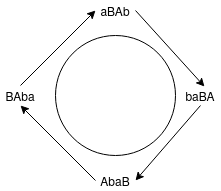
Anyway. We want to explore our tree in a cyclic order of \(a, B, A, b\): we are interested in all four cyclic permutations \(B, A, b, a\),\(A, b, a, B\),\(b, a, B, A\),\(a, B, A, b\). We can now think of turning left and right as choosing a different direction in our cyclic order.

Say you have a word \(wB\), meaning that it ends in B, and that the last generator you used is B, meaning that the inverse of this path is \(b\). Since \(b, a, B, A\) is a cyclic permutation of \(a, B, A, b\), we know that the forward direction, in inverse order must be \(a, B, A\).

Now, if we move always right, we would chose the A branch. After choosing, the \(A\) branch we would chose the next cyclic permutation, or \(B, A, b, A\), meaning that our next most right hand generator would be \(B\). If we must go up a level, meaning that we can’t chose \(B\) we chose the next rightmost turn possible, or \(A\). If we can’t again, we chose \(b\), and if we have exhausted all of our options, we must go back a level and try the next rightmost possible turn.

This cyclic permutation bodes very well with our beloved modulo operator. We even have placed the generator in such a way that the index of a generator and its inverse is simply \(i_{\bar{gen}} = i_{gen} + 2 % 4\). What a coincidence. All of this text just means something simple: given an index \(i\) the next generators are just given by \(i - 1, i, i + 1\) modulo 4.

What are we plotting ?

With the BFS algorithm, what we essentially did was applying a Möbius transform on each of the 4 circles of the initial Schottky array. As it turns out, we don’t need to do apply this transform to a specific circle. What we could do, is simply chose a seed point \(P\) in the initial Schottky circles, and apply the transform not to the entire circle, but simply to this point, saving us some computations. This also means that if we chose seed two points \(P\) and \(Q\) that are initially in the same tile, then their image by the word \(W\) will be very close. Sadly, this means that we need to chose initial points which are in a tile mapped by a word. Choosing random points to apply this transformation too is a bad idea since most of them won’t be in those tiles, and in longer word the tiles shrink to nothing. After all we want to plot the limit set of a particular group, i.e what happens when the initial Schottky circles are transformed by long words. With the BFS, we usually do this at each step, but this is fairly slow, and also require the position and radius of all initial circles, which might not be straightforward to obtain using more complicated recipes (or no recipes at all). So, we need a way to have points \(P\) which are always in the initial Schottky tiles.

The answer here is to take advantage of an equivalency between fixed points of generators and limit points. But we first need to know how to deal with those infinite words that we so desperately need to draw limit sets. I’m gonna paraphrase a bit here, so bear with me.

Rules of da Game

There are a few rules that we’ll take advantages when exploring longer and longer words. Ideally we’d like to explore infinitely long words, but I can’t wait that long so we’ll approximate them using those simple rules:

• Words that begin the same and stay the same for a long time have close limit points

• If \(P\) is a limit point, then \(W(P)\) is the infinite word made by fusing \(W\) in front of \(P\) and making the necessary cancellations

• Infinite words with repetends correspond to fixed points of transformations in the group. For example if \(W\) and \(V\) are finite reduced words, we have:

  • If the first and last letter of \(W\) are not inverses of each other, then \(\bar{W} = \text{Fix}^+ (W)\)

  • If the first and last letter of \(W\) are inverses of each other then \( \text{Fix}^+ (W)\) is the infinite reduced word made from \(\hat{W}\) by making all the necessary cancellations at the join

  • With the necessary cancellations done, \(V\hat{W} = \text{Fix}^+ (VWV^-1) = V \text{Fix}^+ (W)\) =

Special words for special people

Alright, we’re back in the game, and we know the rules. If we need to plot the point \(P\) associated to an infinite word \(BBBaabAABB…\), using the first rule we know that \(P\) will be close to any limit point whose word also begin with \(BBBaabAABB…\) like \(BBBaabAABB\hat{a}\). Using the third rule, we also know that \(BBBaabAABB\hat{a} = BBBaabAABB \text{Fix}^+ (a)\). And that’s it !

Our algorithm will basically explore all reduced words of a maximum length which afterwards consist of simply a repetition of a single letter. Another way to put it is that we’re looking at all the possible points which are \(W(Fix^+ (a), W(Fix^+ (b), W(Fix^+ (A), W(Fix^+ (B)\). Choosing a higher maximum word length will let us draw much more points, increasing exponentially, and adding much more details.

But nothing is telling us that those special words cannot be longer than a single symbols. Actually, when we’ll take a look at “accidents”, which are Apolonius Packing that are related to fractions (and irrationals), those special words can be much longer. Fortunately Ceendras Pearl also include an automated special word generator that also includes them in the exploration process. Yes this took me way too much time.

Endpoints Conditions

So we know what branch to take when exploring. How do we know when to stop ? The first thing that could come to mind is simply stop using a maximum depth level. Once we have reached this depth, immediately come one level up and start again. But we could use another trick. We could stop once the image of a few fixed points are close enough together, let’s say under an \(\varepsilon\). Using the BFS algorithm, we used to apply the obtained Mobius Transform onto a circle, and plot this. But we don’t have those initial circles anymore, and this operation was fairly expensive. An easy fix to this is to simply draw a point only if the newly obtained point is at a distance smaller than an \(\varepsilon\) of the old point. If yes, the new point becomes the old point and we start again. The first old point should be the fixed point of the first generator used, so that we can start the show. Drawing a line in this context is trivial: simply connect the old point and the new point if their distance \(< \varepsilon\)

This is fine, but it comes with a significant problem: the limit set can be very twisty, and sometimes the distance between the fixed points can be smaller than an \( \varepsilon\) leading up to an undesirable early termination. This is where we use our special words. We construct a 2D table with all the cyclic permutations of the special words and store them by the last generator used. Our will therefore table will be 4 by len(specialWord), because we have 4 generators, and the number of cyclic permutations is equal to the length of the word. Note that each index on this table won’t actually have the same number of elements, since all generators won’t necesseraly appear the same number of time in the special word. For example the word \(aaBABab\) has 3 \(a\), 2 \(B\), 1\(A\) and 1 \(b\). We also store the inverse of all the permutations of the special word, where the inverse is basically replacing all the generators in the word by their inverse. Finally, we compute the fixed points of all those words.

So if the special word is \(aaB\), our table will have the following element: the index 0, corresponding to the generator \(a\) will contain the fixed points for \({aBa, Baa}\). Index 1 for generator \(b\) will contain the F.P for \(AAb\), index 2 (generator \(A\)) will contain the F.P. of \({bAA, AbA}\) and finally index 3 (generator \(B\)) will contain the F.P. of \(aaB\)

Pfew, that’s a lot to take in ! Now that we have our table we are ready to check the endpoint. When we explore in depth first, we first go forward in the tree, and each time we move further in levels, we check if we can still go forward by checking the distance between the currently explored word and the table of fixed point we have pre-generated. We get the index by checking the last generator used in the word, and then we compute the distance between all the fixed points of that index multiplied by the current word. If all the distances are under an epsilon, we can draw a line between those points. For example if our currently explored word is \(aBBBBabbbAAbAAba\), the last used generator is \(a\). We will compute the points tha

Faster, faster !

Now this is all fine and dandy, but we’re quite slow. Is there anything we could optimise ? The obvious idea would be to parallelize this affair. Turns out it’s fairly easy to do. Since we explore branches of the tree, and that this exploration is entirely independent from one another, we can simply use multithreading to speed up our exploration. The easiest way would be to use on thread per initial branch: each thread would be responsible for the exploration of every word starting with a specific letter. We end up with a 4x boost in exploration speed, although with a 4x boost in memory, since every array used in the exploration is quadrupled. However, the memory cost of ceendras is actually pretty light, since we are using just a few hundred-elements long complex array.

The implementation of this idea was actually easier that thinking about it. Since every branch is actually entirely independent, we can just specify the branch to explore by giving it another end condition: usually the program would stop once it has done an entire cycle through the generators, or abAB, but now we just ask it to stop once the first letter would change.