Bifurcation Diagrams

This time we’re gonna talk about things I know a little bit more about : bifurcation diagrams and iterated functions. The code is available here

Bifurcation diagrams show the behavior of a function $ f: \mathbb{R} \rightarrow \mathbb{R} $, with a real parameter under iteration. Iteration simply means “plugging the output into the input”: a feedback if you will. Iterating from a “seed” $p$, the function can converge to a value (i.e. a fixed point), explode into $\infty $, or go into a cycle. A cycle can have a period, which is the number of iteration you need to do to come back to the original value. In other words, a periodic point $p$ of period $k$ is defined as $f^k(p) = p$, with $k$ being the smallest integer with which this condition is true. Here, $f^k$ simply means iterating the function $k$ times.

Sometimes, the function will go into an “aperiodic cycle”, where the function won’t come back to a fixed point. This is chaotic behavior. A chaotic orbit will never visit a point which it has already been to.

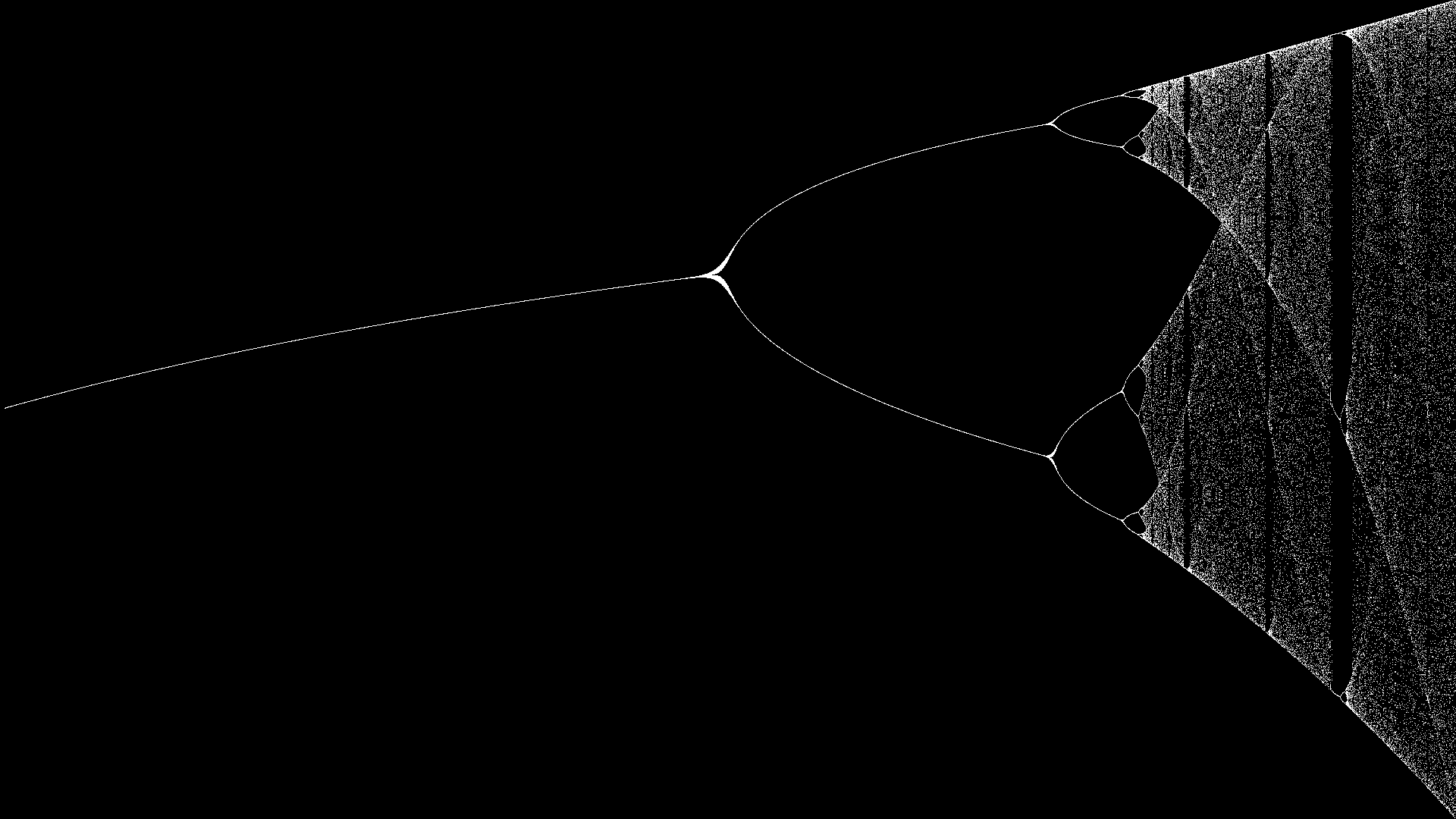
Enough chit-chat. In this bifurcation diagram, we see if our function converge to a fixed point, or go into an (a)-periodic orbit. We can iterate whatever function we like (well, not quite; it has to be a real function and have only one real parameter) but usually we show the classic logistic function:

$$ f_{n+1}(x) = ax(1-x) $$

Note that this function is actually a second degree polynomial.

On the $x$ axis, we vary the parameter $a$ from 2 to 4, and we iterate the function, starting from a point $p$. After a fixed number $k$ of iteration to let the function stabilise itself we start plotting points whose coordinates are now $ (a, f^n(p))$, with $K < n < M$. And tada, we have a bifurcation diagram.

We can see the classic Road To Chaos, with period doubling happening quicker and quicker. First, $f$ converge to a fixed point, then it splits into a 2-cycle. Then a 4-cycle, a 8-cycle… faster and faster. The rate at which those bifurcation occurs is the Feigenbaum $\delta$ constant. Then chaos, or a big blob of white on the screen.

This behavior is linked to the number of solution to the equation $f^k(x) = x$. As $f$ is a 2nd degree polynomial, and since the iterate of a polynomial is also a polynomial, we will always have $2^K$ solutions. However, most of them will be in the complex plane. Since our seed is real, we need real solutions. Luckily, as the parameter $a$ increase, the solutions becomes real for higher and higher iteration number, and our function gradually becomes chaotic.

Now of course you don’t have to use the logistic function. Here’s the bifurcation diagram of the “Gauss function”.

$$ f_{x+1} = exp[\alpha x_n^2] + \beta $$

Now we’ve tricked out a bit here, since we have two parameters: every frame shows a different value of $\alpha$, ranging $[4;7]$, and the $ x$ axis is the $ \beta $ parameter in the range $[-1;1]$.

This won’t be the last time I’m gonna talk about bifmaps. There’s great stuff to be done in here!