Tiling Generation: First Impact

For the past few months, I have been working on Mortier, a powerful tesselation generator written in Python. It is able to generate k-uniform tilings, Penrose tilings and even some Hyperbolic tilings. It also implements the “Polygon in Contact” algorithm which creates some intricate patterns that are similar to some Islamic Art motifs.

But, what even is a tiling ? What is this “k-uniform” you are talking about ?

Tilings

In it’s most basic form, a tiling is a way to arange shapes so that they cover an area without overlapping. There is a lot of examples of tilings, even just around you. Your flooring might be composed of tiles, or the decorations around your bathrooms might form a tiling. Tiles have been very useful in Human history since you can decorate or fill a space by just applying the same shape (or shapes) over and over again. You can understand frises as some type of tiling as well. A lot of things just compose themselves well.

However, in a more mathematically rigorous sense, we will be restricting the rules a bit. We are interested in tilings that are composed of regular polygons, which are equilateral and equiangle polygons, like the square or the octogon. We will also ask that those polygons be convex. Those tilings have been studied for quite some time, at least since antiquity. The tilings will also be composed “edge to edge”, so you can’t cheat around by sliding one tile around another. Tilings and tesselation are quite closely related, so I also tend to interchange the terms quite a bit.

Regular Tilings

If you use only one shape, it turns out, there is not a lot of tilings you can do. Those are called regular tilings. There is only 3 polygons which are able to be tiled this way: the triangle, the square and the hexagon.

This is due to some very simple fact: at each vertex, the sum of the angle of the polygons composing this vertex must be $2 \pi$. Or, in a more mathematically respectable way:

$$ \sum^n_{i=0} \frac{k_i - 2}{k_i}\pi = 2\pi $$

If you put 6 equilateral triangles, you get $\sum^6_{i=0} \frac{\frac{2}{3} \pi - 2}{\frac{2}{3} \pi} = 2 \pi$, and Bob’s your uncle.

Here, we’ll start to introduce some notations. We’ll use Cundy & Rollet’s notations, since it’s fairly easy to understand. We can indicate the type of tiling by looking at a vertex and identifying which polygons it is composed of. For the triangle tiling, each vertex is composed of 6 triangles. Since a triangle has 3 edges (last I checked), we can then call this vertex something like $(3 \cdot 3 \cdot 3 \cdot 3 \cdot 3 \cdot 3)$, or $(3^6)$ for short. The square tiling is also easy: it is simply $(4^4)$

Unfortunately this equation does not allow for any other configurations other than the one listed. So do we just give up and go home ?

Archimedean or Uniform tilings

No, we don’t. As life teaches us, when there is too much restrictions we must rebel. If we allow ourselves to use different regular polygons at one vertex, we are able to create much more diverse tilings. We restrict ourselves we vertex transitivity, meaning that for each pair of vertices there exists a symmetry operation mapping the first vertex to the second. Those relaxed conditions allows us to find 8 more tilings.

However, we start running in some difficulties. While some of those combinations might make sense locally, whereas they meet at a point with no overlapping or gaps, they do not tile the plane by themselves. For example $(3 \cdot 3 \cdot 4 \cdot 12 )$, shown here.

So, we still find ourselves frustrated. We found some working solutions for our equations, but we can’t use them. We now need to further relax our conditions in order to use then.

K-uniform tilings

If we allow ourselves to use multiple configurations to tile the plane, we have much more liberty. We can classify the above tilings by the number of orbits of vertices. A k-uniform tiling has k-orbits. An orbit here is defined in the group theory sense, wherein the orbit of an element $x \in X$ is the set of elements in $X$ which can be moved by the elements in $G$.

Or:

$$ G \cdot x = \{g \cdot x : g \in G\} $$

In other words, if you have one vertex “type”, which can be translated, rotated, reflected or “glide reflected” to another vertex of the same type, and there no other, you have a 1-uniform tiling.

There is 12 1-uniform tilings, which contain the 3 regular tilings and the 8 semi-regular tilings. There is 20 2-uniform tilings, 61 3-uniforms and so on. As you increase the number of orbits, you get much much more possible tilings. In some sense, an $\infty$-uniform tiling is an aperiodic one. You can also group k-uniform tilings with the number of distinct vertex figures.

Tiling generation and Soto-Sanchez Algorithm

“Alright, that’s great and all, but how do we look at them ? I don’t care about this mathematic mumbo jumbo, I just want to look at cool patterns !”, you say, trembling with anger.

I look at you, asking to myself while you would say that while looking at a blog which is explicitely about mathematics.

Mortier implement a very nice algorithm presented in Dr. Sotò Sanchezs Thesis. I’ll present it concisely:

Representation

The first intuition is to realise that tiling comprised of regular polygon have two nice properties:

• Since an edge of a regular polygon must be of length $1$
• They can be only composed of triangles, squares, hexagons, octogons and dodecagons

However, the octogons don’t play nicely with other regular polygons. Since it is not used in higher uniform tilings, we can safely exclude it from our representation.

We can use those properties to derive another representation for the edges. Since the highest number of sides in a regular polygon used in a k-uniform tiling is 12 (the dodecagon), the number of distinct directions an edge can have in one those tiling is then also 12. A regular polygon is equiangle which means that those directions are equally spaced around the circle, and since they are all equilateral it also means that the length of those directions vectors are all the same. A good representation for this would then be the 12th root of unity.

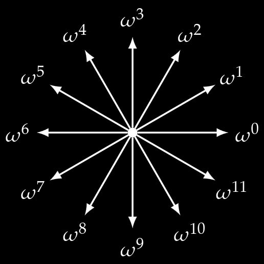
Using those roots, we can also define some kind of “paths”. For example we can consruct a square by adding $w^3 + w^0 + w^9 + w^6$. Starting from the origin, it would look like going east, then north, then west and finally south. You can now represent a square in terms of element in the 12th roots of unity, or as a 12th order polynomial with integer coefficients. In essence, we are able to represent vertices and translation vectors as integers polynomials of $w$, or $\mathbb{Z}[w]$.

In the figure below, we can see one of those path. We can represent the position of one vertex from each other with a polynomial in $w$. For example we have: $$V - O = w_2 + w_{11} + w_1 + w_3 + w_2 + w_5 + w_6$$ Or $$V - O = w_1 + 2 w_2 + w_3 + w_4 + w_5 + w_6 + w_{11}$$

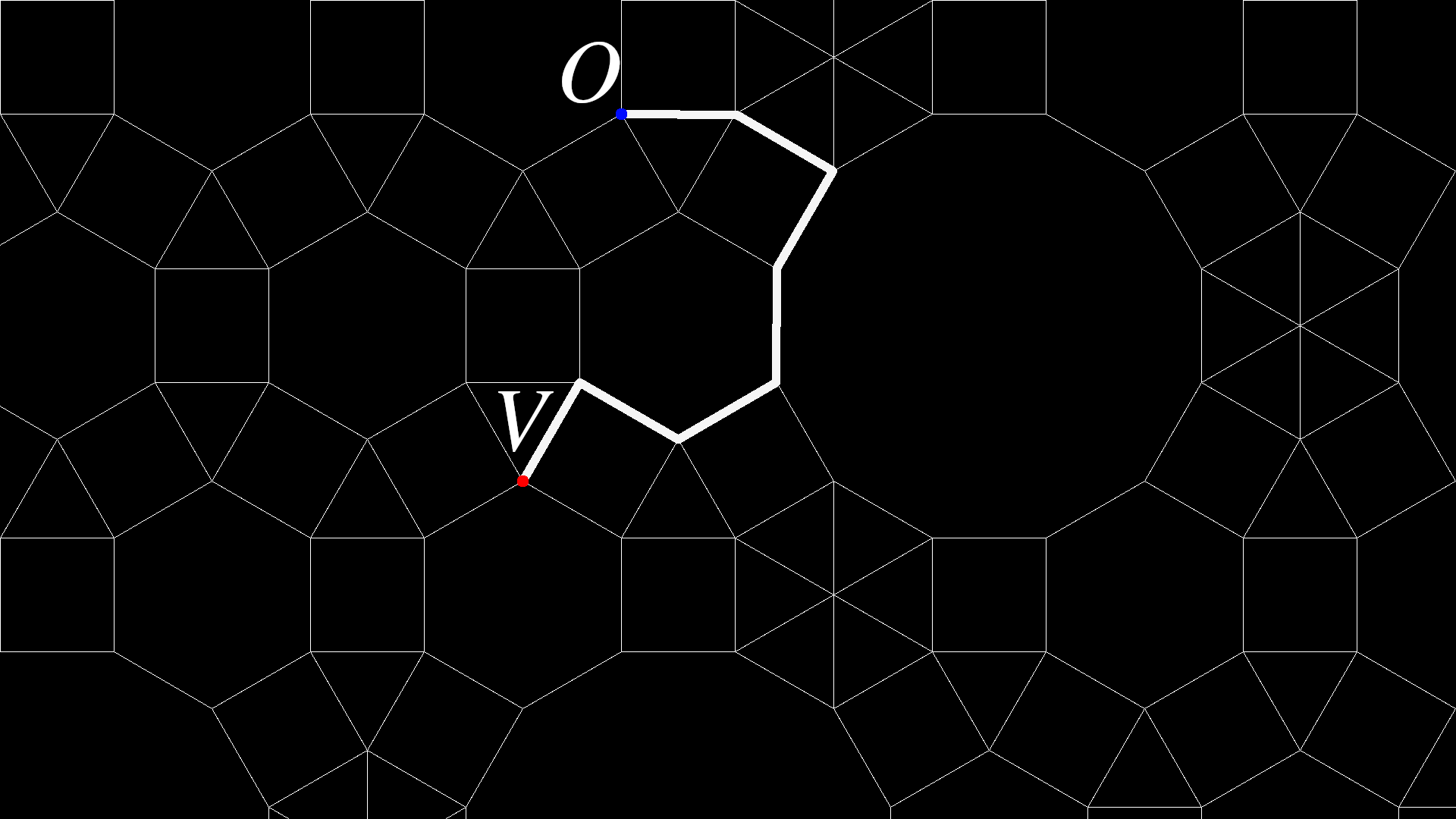
However, this representation is not unique. There might be multiple “paths” from one point to another. By reducing the polynomial representation by mod $(w^4 - w^2 + 1)$, the minimal polynomial in the field, we are able to obtain a vector in $\mathbb{Z}[w]$ that uniquely define a point in $\mathbb{R}^2$. For our representation above, we can reduce it to $2w_3 + 3 w_2 - 1$. This means that our original polynomial can be represented by a integer coefficient polynomial of order 3. When used as coordinates we obtain an unique 4-integer vector for every vertex in the tiling. In this sense, we can also think about them as translation vectors.

Generation

To obtain a tiling, we need 2 elements: the translation vectors, and the “seeds”. The translation vectors define the fundamental domain in which the tiling lives. This cell is a parallelogram that, when tiled, reproduce the tiling inside of it. The seeds are the initial vertices inside the fundamental domain. Those elements are pre-computed, and are extracted from a database of tilings. Both the translation vectors and the seeds are represented using the $\mathbb{Z}[w]$ coordinates, since it allows us for faster (and exact) computation.

We first use the translation vector to “pre-tile” our fundamental domain. We tile it once for every 8 directions (think of it as the Moore Neighborhood of the domain), since some of the seeds might connect to other seeds which are outside of the domain, but just translated once. While doing this, we construct an hashtable. Since the representation of each vertex/seed is unique, we can compute a hash of the representation to enhance neighborhood checking, as we’ll see.

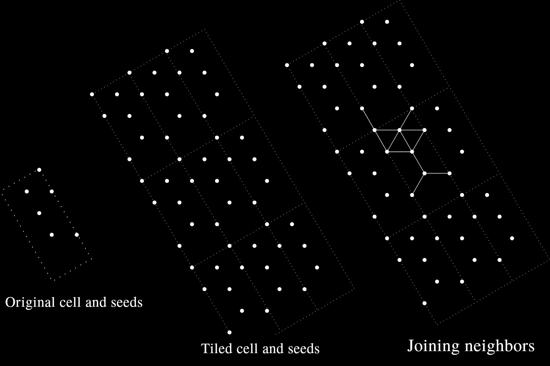
Then, we iterate over all seeds. For each seed $v$, we check around to see if there is another seed at distance 1. We do so by iterating through the 12 power of $w$ and adding it $v$, or simply looking at the set $\{v + w^k, \forall k \in \{0, 1, \dots, 12\}\}$. Remember, for tilings made up of regular polygons, every edge of every polygon is of length 1. Since the representation of each vertex/seed is unique and exact, we can use our hashtable for this check. We simply look in our hashtable if the hash of $v + w^k$ exists. If it does, we just join the two by an edge, and we’re done. We then can simply tile this “tiling skeleton” along the translation vector to reconstruct the entire tiling.

This representation also allows for easily creating (and identifying) faces from edges, but I won’t get into that, since we’re starting to run a bit long. Mortier implements all of this and quite more, so be sure to experiment with it ! I’ll do another post to explain some more cool stuff you are able to do with it.